GridWorld, Policy Evaluation, Monte Carlo, and TD Control
This project implements a compact but expressive GridWorld environment and a suite of control algorithms: exact policy evaluation via a linear system, value iteration, on/off-policy Monte Carlo control, and on/off-policy Temporal-Difference control (SARSA and Q-learning). The work focuses on clarity of the Markov Decision Process dynamics, careful state-value and action-value updates, and practical visualization of convergence and policies.
- Environment: tabular GridWorld with bounce-on-walls/blocks, terminal goal/fire states, step cost, and optional stochasticity.
- Evaluation/Control: linear system for V^π, value iteration, every-visit Monte Carlo (on/off-policy), SARSA, and Q-learning.
- Visualization: convergence curve, heatmap of V(s), and final greedy policy arrows.
Here is the full report:
Links: Notebook, Report PDF
GridWorld: States, Actions, Transitions, Rewards
Actions are enumerated and mapped to readable symbols:
class Action(IntEnum):
    up = 0
    right = 1
    down = 2
    left = 3

action_to_str = {
    Action.up : "up",
    Action.right : "right",
    Action.down : "down",
    Action.left : "left",
}
Transitions “bounce” off walls and blocked cells, preserving the current state if movement would exit bounds or hit a block:
    def _state_from_action(self, state, action):
        """
        Gets the state as a result of applying the given action
        """
        # The state passed must be valid to start with
        assert self._inbounds(state)
        # Get the index of the new state given an action
        match action:
            case Action.up:
                new_state = state - self._width
                if not self._inbounds(new_state): # Bounce off the top wall
                    return state
            case Action.down:
                new_state = state + self._width
                if not self._inbounds(new_state): # Bounce off the bottom wall
                    return state
            case Action.left:
                new_state = state - 1
                if new_state % self._width == self._width - 1: # Bounce off left wall
                    return state
            case Action.right:
                new_state = state + 1
                if new_state % self._width == 0: # Bounce off right wall
                    return state

        if new_state in self._blocked_cells: # Bounce off blocked cells
            return state

        return new_state
Reward shaping is simple: goal and danger states are terminal with specified rewards; non-terminal states have a small step cost:
def get_reward(self, state):
    """
    Get the reward for being in the current state
    """
    # The state passed must be valid to start with
    assert self._inbounds(state)
    # Reward is non-zero for danger or goal
    if state == self._goal_cell:
        return self._goal_value
    elif state in self._danger_cells:
        return self._danger_value

    return -0.1 # Default reward for being in a non-terminal state
Stochasticity is optional. Deterministic transitions return a single next state with probability 1; with noise, the chosen action is followed with probability 1−noise and other actions are taken proportionally:
def get_transitions(self, state, action, deterministic=True):
    """
    Get a list of transitions as a result of attempting the action in the current state
    Each item in the list is a tuple, containing the probability of reaching that state and the state itself
    """

    # The state passed must be valid to start with
    assert self._inbounds(state)

    # Find possible next actions
    possible_actions = self.get_actions(state)

    # Selecting an action isnt noisy, meaning there is no exploration
    if not deterministic:
        p_desired_action = 1 - self._noise
        p_undesired_action = (self._noise) / (len(possible_actions) - 1)
        # The probability of choosing a different action is (1 - probability of choosing the desired action)
        # divided by the number of undesired possible actions

        transition_list = []
        for possible_action in possible_actions:
            if possible_action == action:
                transition_list.append(
                    (self._state_from_action(state, action), p_desired_action)
                )
            else:
                transition_list.append(
                    (self._state_from_action(state, possible_action), p_undesired_action)
                )

        # Since all actions are possible, the return will always look like this:
        # [
        #     (new_state, p(new_state|action_1)), # Chosen action (passed argument)
        #     (new_state, p(new_state|action_2)), # Noisy action
        #     (new_state, p(new_state|action_3)), # Noisy action
        #     (new_state, p(new_state|action_4))  # Noisy action
        # ]
        return transition_list

    # Deterministic transition probability. The action will always take you to the next cell,
    # Unless you hit a wall, which will result in you being in the same state. Happens with p(1).
    return [(self._state_from_action(state, action), 1)]
Exact Policy Evaluation via Linear System
For a uniform random policy, the Bellman equations V = R + γ P_π V are assembled into A V = b and solved directly:
def solve_linear_system(self, discount_factor=1.0):
    """
    Solve the GridWorld using a system of linear equations corresponding to:

        V^π(s) = Σ_a π(a|s) Σ_{s',r} p(s', r | s, a) [r + γ V^π(s')]

    for all non-terminal states s.

    Parameters:
    -----------
    discount_factor : float
        The discount factor (γ) for future rewards.
    """


    # Initialize matrix A to ones, vector b to solve A * V = b for the value vector V = [V(s_0), ..., V(self._num_states)].
    A = [[0.0 for _ in range(self._num_states)] for _ in range(self._num_states)]
    b = [0.0 for _ in range(self._num_states)]


    # Loop over all states in self._grid_values
    for state in range(self._num_states):
        A[state][state] = 1.0 # Set the diagonal to 1 to isolate V(s) on the left-hand side. For terminal states, this yields V(s) = R(s).
        b[state] = self.get_reward(state) # Set reward of the state

        # If 's' is terminal, V(s) = R(s) since we don't transition anywhere after.
        # So the row is simply:  A[s][s] = 1,  b[s] = R(s).
        if self.is_terminal(state):
            continue


        # Sum up all transitions from s under each action a.
        actions = self.get_actions(state) # All the actions which can be taken from a state
        pi_sa = 1.0/len(actions)  # π(a|s) = 1/4 since all action probabilities are uniformly distributed

        for possible_action in actions:

            # transitions = iterator through dicts of {next_state, probability_of_next_state}
            transitions = self.get_transitions(state, possible_action)

            # For each possible next state s_next and its corresponding transition prob p_s_next, incorporate the reward + γ V^π(s').
            # In the determinitic case, we will always transition to the intended next state with p(1) unless we hit a wall, in which case
            # we stay in the same state.
            for s_next, p_s_next in transitions:
                r_snext = self.get_reward(s_next) # The reward of being in next state.

                # Add the reward of s_next to b[state].
                # b[s] accumulates: Σ_{a} π(a|s) Σ_{s'} p(s'|s,a) * R(s')
                # summation(actions for loop):
                #   1/len(actions) * summation(transitions for loop):
                #       Transition probability from state to s_next (1 in this deterministic case) * reward of being in s_next
                b[state] += pi_sa * p_s_next * r_snext

                # Subtract the discounted transition from A[s][s_next].
                # A[s][s_next] accumulates: - γ * π(a|s) * p(s'|s,a)
                # summation(actions for loop):
                #   summation(transitions for loop):
                #       negative discount factor * p(selecting this possible_action) * p(s_next given possible_action and state)
                # This accumulation accounts for all actions and transitions from state 'state' that lead to s_next.
                A[state][s_next] += -1 * discount_factor * pi_sa * p_s_next

    # Convert to numpy array and solve
    # print(f"MATRIX:\n{A}")
    A = np.array(A)
    b = np.array(b)
    V_solution = np.linalg.solve(A, b)

        # Store the resulting values back into self._grid_values.
        self._grid_values = V_solution.tolist()

        # Each V(s) now satisfies Bellman Eq: V^π(s) = Σ_a π(a|s) Σ_{s'} p(s'|s,a) [ R(s') + γ V^π(s') ]


    # All the following control algorithms will be implemented on every visit
This serves as a correctness baseline for the dynamic-programming and learning methods below.
Value Iteration (Greedy Policy Improvement)
Each sweep computes the best action value from state s and updates V(s) accordingly until max delta < tolerance:
def value_iteration(self, discount_factor=1.0, tolerance=0.1, deterministic=True):
    policy = [None for _ in self._grid_values]
    iteration_info = []
    while True:
        curr_grid_values = self.create_next_values()
        delta = 0.0
        for state in range(len(curr_grid_values)):
            if self.is_terminal(state):
                curr_grid_values[state] = self.get_reward(state)
                continue
            v_state_curr = self.get_value(state)
            best_action_ev = float('-inf')
            for possible_action in self.get_actions(state):
                action_transitions = self.get_transitions(state, possible_action, deterministic=deterministic)
                current_action_ev = 0.0
                for next_state, p_next_state in action_transitions:
                    current_action_ev += p_next_state * (self.get_reward(next_state) + discount_factor * self.get_value(next_state))
                if current_action_ev > best_action_ev:
                    best_action_ev = current_action_ev
                    policy[state] = action_to_str[possible_action]
            curr_grid_values[state] = best_action_ev
            delta = max(delta, abs(v_state_curr - best_action_ev))
        self.set_next_values(curr_grid_values)
        iteration_info.append({ 'delta': delta, 'policy': policy.copy(), 'grid_values': self._grid_values.copy() })
        if delta < tolerance:
            break
    return iteration_info
On-Policy Monte Carlo Control (Every-Visit, ε-Soft)
Episodes are generated using the current ε-soft policy; returns are averaged to update Q, then the policy is improved to be ε-soft greedy w.r.t. Q:
def on_policy_montecarlo_control(self, num_episodes, discount_factor=1.0, epsilon=0.1):
    """
    On-Policy Montecarlo Control Algorithm
    Following the psuedocode in textbook chapter 5.4 page 101
    """

    # Number of states and actions

    # State-action value function Q(s, a)
    Q = [[0.0 for _ in range(self._num_actions)] for _ in range(self._num_states)]  # Q(s, a)

    # State-action rewards function R(s, a)
    R = [[[] for _ in range(self._num_actions)] for _ in range(self._num_states)]  # R(s, a)

    # Initialize the policy π(s) so each action is equally probable in every state
    policy = [[1/self._num_actions for _ in range(self._num_actions)] for _ in range(self._num_states)] # π(s)

    iteration_info = [] # Holds information about each iteration in the optimization
    iteration_count = 0


    # Generate an episode using the current policy and e-soft exploration
    for _ in range(num_episodes):
        episode = [] # The episode is a list of tuples (state, action, reward)
        delta = 0.0 # Keep track of the maximum difference between a state and its update, for all states in the episode
        visited_states = set()

        # Generate an episode using the current policy π:

        curr_state = self._start_cell # Start from the start state
        # Loop until we reach a terminal state or the episode length limit
        while not self.is_terminal(curr_state) and len(episode) < self._episode_limit:
            # Sample an action from the policy, accounting for probability
            action = np.random.choice(self._num_actions, p=policy[curr_state])

            # Take the action to get to the next state
            next_state = self._state_from_action(curr_state, action)

            # Get the reward for the next state
            reward = self.get_reward(next_state)

            # Record the tuple (state, action, reward) in episode
            episode.append((curr_state, action, reward))

            # Record that we vitited the state
            visited_states.add(curr_state)

            # Move to the next state
            curr_state = next_state


        # For each state-action pair in the episode, update the state-action value function Q.
        for t, (state, action, reward) in enumerate(episode):
            # Calculate the accumulated reward for this step. The accumulated reward is the
            # current reward, plus the discounted reward for the next steps
            accumulated_reward = reward

            next_steps = episode[t + 1:]
            for t_i, (_, _, reward_t_i) in enumerate(next_steps, start=1):
                accumulated_reward += discount_factor**(t_i) * reward_t_i

            # Append the accumulated reward to this State-Action pair
            R[state][action].append(accumulated_reward)

            # Incrementally update Q(s,a) by averaging the accumulated reward:

            # Number of times we visited this state action pair
            n_sa = len(R[state][action])
            # What is the average accumulated reward from this state action pair
            avg_accumulated_reward_sa = sum(R[state][action])/n_sa

            # Update Q
            Q[state][action] = avg_accumulated_reward_sa


        # After the episode, policy improvement:
        for state in visited_states:
            # First, update the value of the state:
            old_state_value = self._grid_values[state]
            new_state_value = max(Q[state]) # Value of state is the value of taking the best action
            # Keep track of the biggest change in state value in the episode
            delta = max(delta, abs(old_state_value - new_state_value))
            self._grid_values[state] = new_state_value # Update

            # Next, update the policy to be epislon-soft with respect to the state-action value function Q
            best_action = np.argmax(Q[state])
            for possible_action in range(self._num_actions):
                if possible_action == best_action:
                    policy[state][possible_action] = 1 - epsilon + (epsilon / self._num_actions)
                else:
                    policy[state][possible_action] = epsilon / self._num_actions


        # Record this iteration's information for later analysis:

        # Compute the ideal policy for tracking purposes. For each
        # state, select the action with the highest probability:
        ideal_policy = [action_to_str[Action(np.argmax(state_policy))] for state_policy in policy]
        iteration_info.append({
            'episode': episode,
            'iteration': iteration_count,
            'delta': delta,
            'policy': ideal_policy.copy(), # Copy of the current policy.
            'grid_values': self._grid_values.copy() # Copy of state values for this iteration.
        })
        iteration_count += 1

    return iteration_info
Off-Policy Monte Carlo Control (Ordinary Importance Sampling)
Episodes come from a fixed behavior policy; Q is updated using weighted returns, and the greedy target policy is improved accordingly:
def off_policy_montecarlo_control(self, num_episodes, discount_factor=1.0):
    """
    Off-Policy Monte Carlo Control using Ordinary Importance Sampling.
    This method uses a fixed behavior policy to generate episodes and then updates the Q-values
    and state values based on the returns from those episodes. Follows the psuedocode on page 111
    of the textbook.
    """
    # Initialize state-action value function Q(s,a)
    Q = [[0.0 for _ in range(self._num_actions)] for _ in range(self._num_states)]

    # Initialize cumulative importance-sampling weights C(s,a)
    C = [[0.0 for _ in range(self._num_actions)] for _ in range(self._num_states)]

    # Initialize the target policy π(s) as action 0 for every state
    target_policy = [0 for _ in range(self._num_states)]

    # Behavior policy: I chose a fixed policy, weighting the up and right actions
    # more heavily than down and left since I can see the goal is right and up of the agent.
    # [up, right, down, left]:
    behavior_policy = [0.4, 0.4, 0.1, 0.1]

    iteration_info = []  # To track info for each episode
    iteration_count = 0

    for _ in range(num_episodes):
        episode = [] # The episode is a list of tuples (state, action, reward)
        delta = 0.0 # Keep track of the maximum difference between a state and its update, for all states in the episode
        visited_states = set()

        # Generate an episode using the fixed behavior policy
        curr_state = self._start_cell # Start from the start state
        # Loop until we reach a terminal state or the episode length limit
        while (not self.is_terminal(curr_state)) and (len(episode) < self._episode_limit):
            # Sample an action from the policy, accounting for probability
            action = np.random.choice(len(Action), p=behavior_policy)

            # Take the action to get to the next state
            next_state = self._state_from_action(curr_state, action)

            # Get the reward for the next state
            reward = self.get_reward(next_state)

            # Record the tuple (state, action, reward) in episode
            episode.append((curr_state, action, reward))

            # Record that we vitited the state
            visited_states.add(curr_state)

            # Move to the next state
            curr_state = next_state

        # Initialize the return and cumulative importance weight.
        G = 0.0
        W = 1.0

        # Process the episode in reverse (from last time step to first)
        for t in reversed(range(len(episode))):

            state, action, reward = episode[t]

            G = discount_factor * G + reward

            # Update the cumulative weight and Q using the incremental formula:
            C[state][action] += W

            # Update Q(s,a) using the weighted average of the returns
            Q[state][action] += (W / C[state][action]) * (G - Q[state][action])

            # Update the state value as the max over Q(s,a)
            old_state_value = self._grid_values[state]
            new_state_value = max(Q[state])
            self._grid_values[state] = new_state_value
            delta = max(delta, abs(new_state_value - old_state_value))

            # Update the target (greedy) policy for this state
            best_action = np.argmax(Q[state])
            target_policy[state] = best_action

            # If the action taken in the episode is not the greedy action, break.
            if action != best_action:
                break

            # Update the cumulative importance ratio.
            # Since the target policy is deterministic (greedy), π(a|s)=1 for a=best_action, and 0 otherwise.
            # So, W multiplies by 1/b(a|s) for the action that was actually taken.
            W *= (1.0 / behavior_policy[action])


        # Record this iteration's information for later analysis:

        # Construct an ideal policy
        ideal_policy = [
            action_to_str[Action(target_policy[s])]
            for s in range(self._num_states)
        ]
        # Record iteration information
        iteration_info.append({
            'episode': episode,
            'iteration': iteration_count,
            'delta': delta,
            'policy': ideal_policy.copy(),
            'grid_values': self._grid_values.copy() # Copy of state values for this iteration.
        })
        iteration_count += 1

    return iteration_info
The break enforces ordinary importance sampling with a deterministic greedy target policy.
On-Policy TD Control (SARSA)
Incremental TD updates use the next action from the same ε-greedy policy:
def on_policy_td_control(self, num_episodes, discount_factor=1.0, alpha=0.1, epsilon=0.1):
    """
    On-Policy Temporal Difference Control Algorithm (SARSA).
    Follows the pseudocode from textbook page 130.
    """

    # Initialize state-action value function Q(s,a)
    Q = [[0.0 for _ in range(self._num_actions)] for _ in range(self._num_states)]

    # Initialize the policy π(s) so each action is equally probable in every state
    policy = [[1/self._num_actions for _ in range(self._num_actions)] for _ in range(self._num_states)] # π(s)

    iteration_info = [] # Holds information about each iteration in the optimization
    iteration_count = 0

    # Generate an episode using the current policy
    for _ in range(num_episodes):
        episode = []        # Will store (state, action, reward) for this episode
        delta = 0.0         # Track the maximum change in state-value for this episode
        visited_states = set()


        # Generate an episode using the current policy π:

        curr_state = self._start_cell # Start from the start state

        # Choose A from S using ε-greedy policy derived from Q
        curr_action = np.random.choice(self._num_actions, p=policy[curr_state])

        # Loop until we reach a terminal state or the episode length limit
        while not self.is_terminal(curr_state) and len(episode) < self._episode_limit:
            # Take action A, observe R and S'
            next_state = self._state_from_action(curr_state, curr_action)
            reward = self.get_reward(next_state)

            # Record (S, A, R) in the episode
            episode.append((curr_state, curr_action, reward))
            visited_states.add(curr_state)

            # If S' is terminal, then A' = None
            if self.is_terminal(next_state):
                next_action = None
            else:
                # Choose A' from S' using ε-greedy policy derived from Q
                next_action = np.random.choice(self._num_actions, p=policy[next_state])

            # TD update:
            old_q = Q[curr_state][curr_action]
            future_q = 0.0 if (next_action is None) else Q[next_state][next_action]
            td_target = reward + discount_factor * future_q
            Q[curr_state][curr_action] += alpha * (td_target - old_q)

            # Track the max change in Q to help measure convergence
            delta = max(delta, abs(Q[curr_state][curr_action] - old_q))

            # Update the current state
            curr_state = next_state
            # Update the current action
            curr_action = next_action

        # After the episode, policy improvement:
        for state in visited_states:
            # First, update the value of the state
            old_value = self._grid_values[state]
            new_state_value = max(Q[state]) # Value of state is the value of taking the best action
            # Keep track of the biggest change in state value in the episode
            delta = max(delta, abs(new_state_value - old_value))
            self._grid_values[state] = new_state_value  # Update

            # Next, update the policy to be epislon-greedy with respect to the state-action value function Q
            best_action = np.argmax(Q[state])
            for a in range(self._num_actions):
                if a == best_action:
                    policy[state][a] = 1 - epsilon + (epsilon / self._num_actions)
                else:
                    policy[state][a] = epsilon / self._num_actions


        # Record this iteration's information for later analysis:

        # Compute the ideal policy for tracking purposes. For each
        # state, select the action with the highest probability:

        # Construct the ideal (greedy) policy for visualization
        ideal_policy = [
            action_to_str[Action(np.argmax(Q[s]))] for s in range(self._num_states)
        ]

        # Store iteration info for analysis
        iteration_info.append({
            'episode': episode,
            'iteration': iteration_count,
            'delta': delta,
            'policy': ideal_policy.copy(),
            'grid_values': self._grid_values.copy()
        })
        iteration_count += 1

    return iteration_info
Off-Policy TD Control (Q-learning)
Updates are bootstrapped against the greedy value at the next state, independent of the behavior policy:
def off_policy_td_control(self, num_episodes, discount_factor=1.0, alpha=0.1, epsilon=0.1):
    """
    Off-Policy Temporal Difference Control Algorithm (Q-learning).
    Follows the pseudocode from textbook page 131.
    """

    # Initialize state-action value function Q(s,a)
    Q = [[0.0 for _ in range(self._num_actions)] for _ in range(self._num_states)]

    # Initialize the policy π(s) so each action is equally probable in every state
    policy = [[1/self._num_actions for _ in range(self._num_actions)] for _ in range(self._num_states)] # π(s)

    iteration_info = [] # Holds information about each iteration in the optimization
    iteration_count = 0

            # Generate an episode using the current policy
    for _ in range(num_episodes):
        episode = []        # Will store (state, action, reward) for this episode
        delta = 0.0         # Track the maximum change in state-value for this episode
        visited_states = set()


        # Generate an episode using the current policy π:
        curr_state = self._start_cell # Start from the start state

        # Loop until we reach a terminal state or the episode length limit
        while not self.is_terminal(curr_state) and len(episode) < self._episode_limit:
            # Choose A from S using ε-greedy policy derived from Q
            curr_action = np.random.choice(self._num_actions, p=policy[curr_state])

            # Take action A, observe R and S'
            next_state = self._state_from_action(curr_state, curr_action)
            reward = self.get_reward(next_state)

            # Record (S, A, R) in the episode
            episode.append((curr_state, curr_action, reward))
            visited_states.add(curr_state)

            # Q-learning Update off policy
            old_q = Q[curr_state][curr_action]
            max_q_next = 0.0 if self.is_terminal(next_state) else max(Q[next_state])
            td_target = reward + discount_factor * max_q_next
            Q[curr_state][curr_action] += alpha * (td_target - old_q)

            # Track the max change in Q to help measure convergence
            delta = max(delta, abs(Q[curr_state][curr_action] - old_q))

            # Move on to next state
            curr_state = next_state

        # After the episode, policy improvement:
        for state in visited_states:
            # First, update the value of the state
            old_value = self._grid_values[state]
            new_state_value = max(Q[state]) # Value of state is the value of taking the best action
            # Keep track of the biggest change in state value in the episode
            delta = max(delta, abs(new_state_value - old_value))
            self._grid_values[state] = new_state_value  # Update

            # Next, update the policy to be epislon-greedy with respect to the state-action value function Q
            best_action = np.argmax(Q[state])
            for a in range(self._num_actions):
                if a == best_action:
                    policy[state][a] = 1 - epsilon + (epsilon / self._num_actions)
                else:
                    policy[state][a] = epsilon / self._num_actions

        # Construct the ideal (greedy) policy for visualization
        ideal_policy = [
            action_to_str[Action(np.argmax(Q[s]))] for s in range(self._num_states)
        ]

        # Store iteration info for analysis
        iteration_info.append({
            'episode': episode,
            'iteration': iteration_count,
            'delta': delta,
            'policy': ideal_policy.copy(),
            'grid_values': self._grid_values.copy()
        })
        iteration_count += 1

    return iteration_info
Visualization and Experiments
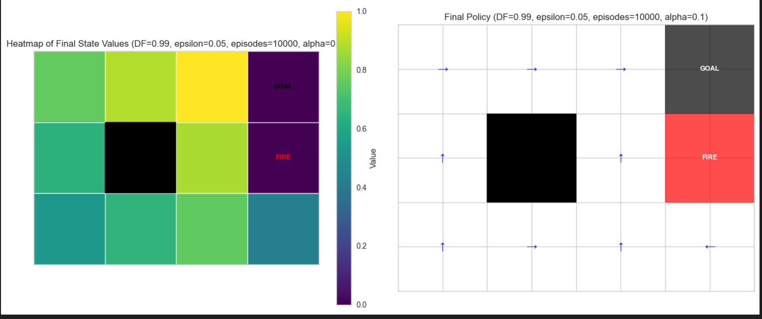
A single helper renders three panes: convergence (max delta per iteration/episode), heatmap of V(s), and a grid of arrows for the final greedy policy. Blocked cells are black, danger cells marked red, and the goal cell annotated. Parameters (discount factor, tolerance, noise, ε, α, episodes) are shown in the title for quick comparison. This is how I generated the visualizations
The notebook varies discount factors, ε, α, and number of episodes to examine stability and convergence speed across Monte Carlo and TD methods.
Takeaways
- Dynamics matter: bounce-on-walls/blocks and step costs shape value propagation and optimal paths.
- Exploration vs. exploitation: ε affects both Monte Carlo and TD behavior; SARSA is on-policy and more conservative than Q-learning near hazards.
- Baselines are useful: the linear solve and value iteration provide targets to sanity-check learning methods.
The full code and plots are in the notebook; the PDF above summarizes results and comparisons across methods and settings.